use of the Event Hub enqueuedTime timestamp instead of NOW() in the INSERT statement (yes, I know, using NOW() did not make sense 😉)
make the code idempotent to handle duplicates (basically do nothing when a unique constraint is violated)
In general, I prefer to use application time (time at the event publisher) versus the time the message was enqueued. If you don’t have that timestamp, enqueuedTime is the next best thing.
How can we optimize the function even further? Read on about the cardinality setting!
Event Hub trigger cardinality setting
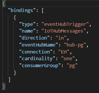
Our JavaScript Azure Function has its settings in function.json. For reference, here is its content:
Clearly, the function uses the eventHubTrigger for an Event Hub called hub-pg. In connection, EH refers to an Application Setting which contains the connections string to the Event Hub. Yes, I excel at naming stuff! The Event Hub has defined a consumer group called pg that we are using in this function.
The cardinality setting is currently set to “one”, which means that the function can only process one message at a time. As a best practice, you should use a cardinality of “many” in order to process batches of messages. A setting of “many” is the default.
To make the required change, modify function.json and set cardinality to “many”. You will also have to modify the Azure Function to process a batch of messages versus only one:
Processing batches of messages
With cardinality set to many, the IoTHubMessages parameter of the function is now an array. To retrieve the enqueuedTime from the messages, grab it from the enqueuedTimeUtcArray array using the index of the current message. Notice I also switched to JavaScript template literals to make the query a bit more readable.
The number of messages in a batch is controlled by maxBatchSize in host.json. By default, it is set to 64. Another setting,prefetchCount, determines how many messages are retrieved and cached before being sent to your function. When you change maxBatchSize, it is recommended to set prefetchCount to twice the maxBatchSize setting. For instance:
It’s great to have these options but how should you set them? As always, the answer is in this book:
A great resource to get a feel for what these settings do is this article. It also comes with a Power BI report that allows you to set the parameters to see the results of load tests.
Conclusion
In this post, we used the function.json cardinality setting of “many” to process a batch of messages per function call. By default, Azure Functions will use batches of 64 messages without prefetching. With the host.json settings of maxBatchSize and prefetchCount, that can be changed to better handle your scenario.
Several years ago, when we started our first adventures in the wonderful world of IoT, we created an application for visualizing real-time streams of sensor data. The sensor data came from custom-built devices that used 2G for connectivity. IoT networks and protocols such as SigFox, NB-IoT or Lora were not mainstream at that time. We leveraged what were then new and often preview-level Azure services such as IoT Hub, Stream Analytics, etc… The architecture was loosely based on lambda architecture with a hot and cold path and stateful window-based stream processing. Fun stuff!
Kubernetes already existed but had not taken off yet. Managed Kubernetes services such as Azure Kubernetes Service (AKS) weren’t a thing.
The application (end-user UI and management) was loosely based on a micro-services pattern and we decided to run the services as Docker containers. At that time, Karim Vaes, now a Program Manager for Azure Storage, worked at our company and was very enthusiastic about Rancher. , Rancher was still v1 and we decided to use it in combination with their own container orchestration framework called Cattle.
Our experience with Rancher was very positive. It was easy to deploy and run in production. The combination of GitHub, Shippable and the Rancher CLI made it extremely easy to deploy our code. Rancher, including Cattle, was very stable for our needs.
In recent years though, the growth of Kubernetes as a container orchestrator platform has far outpaced the others. Using an alternative orchestrator such as Cattle made less sense. Rancher 2.0 is now built around Kubernetes but maintains the same experience as earlier versions such as simple deployment and flexible configuration and management.
In this post, I will look at deploying Rancher 2.0 and importing an existing AKS cluster. This is a basic scenario but it allows you to get a feel for how it works. Indeed, besides deploying your cluster with Rancher from scratch (even on-premises on VMware), you can import existing Kubernetes clusters including managed clusters from Google, Amazon and Azure.
Installing Rancher
For evaluation purposes, it is best to just run Rancher on a single machine. I deployed an Azure virtual machine with the following properties:
Operating system: Ubuntu 16.04 LTS
Size: DS2v3 (2 vCPUs, 8GB of RAM)
Public IP with open ports 22, 80 and 443
DNS name: somename.westeurope.cloudapp.azure.com
In my personal DNS zone on CloudFlare, I created a CNAME record for the above DNS name. Later, when you install Rancher you can use the custom DNS name in combination with Let’s Encrypt support.
On the virtual machine, install Docker. Use the guide here. You can use the convenience script as a quick way to install Docker.
With Docker installed, install Rancher with the following command:
More details about the single node installation can be found here. Note that Rancher uses etcd as a datastore. With the command above, the data will be in /var/lib/rancher inside the container. This is ok if you are just doing a test drive. In other cases, use external storage and mount it on /var/lib/rancher.
A single-node install is great for test and development. For production, use the HA install. This will actually run Rancher on Kubernetes. Rancher recommends a dedicated cluster in this scenario.
After installation, just connect https://your-custom-domain and provide a password for the default admin user.
Adding a cluster
To get started, I added an existing three-node AKS cluster to Rancher. After you add the cluster and turn on monitoring, you will see the following screen when you navigate to Clusters and select the imported cluster:
Dashboard for a cluster
To demonstrate the functionality, I deployed a 3-node cluster (1.11.9) with RBAC enabled and standard networking. After deployment, open up Azure Cloud shell and get your credentials:
az aks list -o table
az aks get-credentials -n cluster-name -g cluster-resource-group
kubectl cluster-info
The first command lists the clusters in your subscription, including their name and resource group. The second command configures kubectl, the Kubernetes command line admin tool, which is pre-installed in Azure Cloud Shell. To verify you are connected, the last command simply displays cluster information.
Now that the cluster is deployed, let’s try to import it. In Rancher, navigate to Global – Clusters and click Add Cluster:
Add cluster via Import
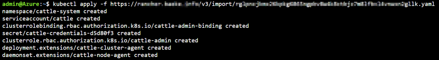
Click Import, type a name and click Create. You will get a screen with a command to run:
Running the command to prepare the cluster for import
Continue on in Rancher, the cluster will be added (by the components you deployed above):
Cluster appears in the list
Click on the cluster:
Top of the cluster dashboard
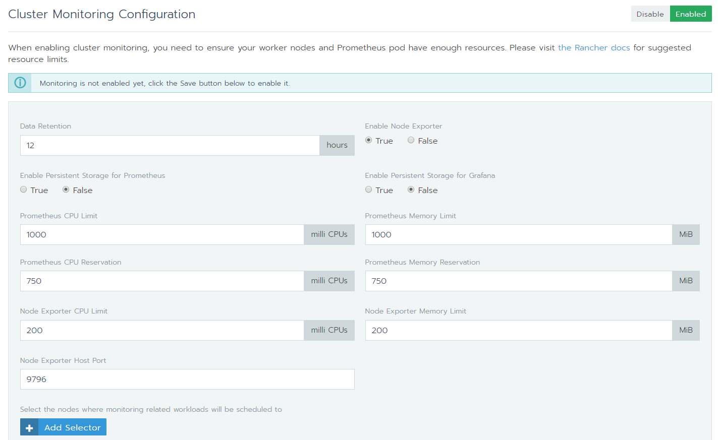
To see live metrics, you can click Enable Monitoring. This will install and configure Prometheus and Grafana. You can control several parameters of the deployment such as data retention:
Enabling monitoring
Notice that by default, persistent storage for Grafana and Prometheus is not configured.
Note: with monitoring enabled or not, you will notice the following error in the dashboard:
Controller manager and scheduler unhealthy?
The error is described here. In short, the components are probably healthy. The error is not related to a Rancher issue but an upstream Kubernetes issue.
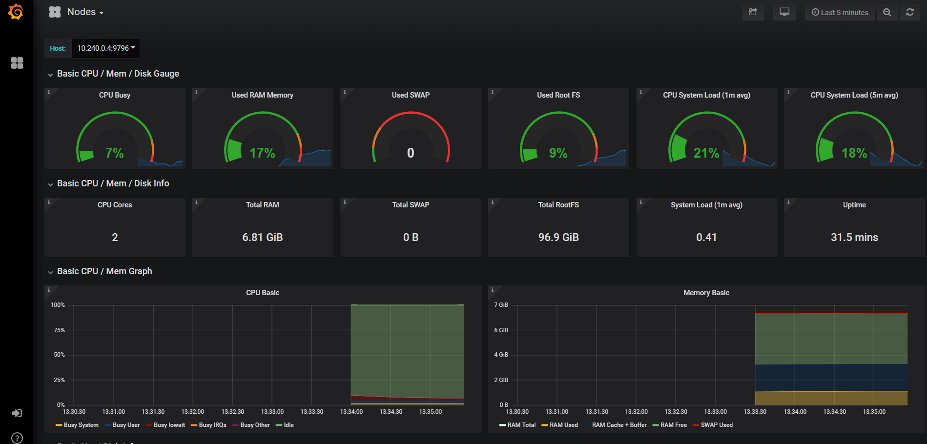
When the monitoring API is ready, you will see live metrics and Grafana icons. Clicking on the Graphana icon next to Nodes gives you this:
Node monitoring with Prometheus and Grafana
Of course, Azure provides Container Insights for monitoring. The Grafana dashboards are richer though. On the other hand, querying and alerting on logs and metrics from Container Insights is powerful as well. You can of course enable them all and use the best of both worlds.
Conclusion
We briefly looked at Rancher 2.0 and how it can interact with a existing AKS cluster. An existing cluster is easy to add. Once it is added, adding monitoring is “easy peasy lemon squeezy” as my daughter would call it! 😉 As with Rancher 1.x, I am again pleasantly surprised at how Rancher is able to make complex matters simpler and more fun to work with. There is much more to explore and do of course. That’s for some follow-up posts!
In an earlier post, I used an Azure Function to write data from IoT Hub to a TimescaleDB hypertable on PostgreSQL. Although that function works for demo purposes, there are several issues. Two of those issues will be addressed in this post:
the INSERT INTO statement used the NOW() function instead of the enqueuedTimeUtc field; that field is provided by IoT Hub and represents the time the message was enqueued
the INSERT INTO query does not use upsert functionality; if for some reason you need to process the IoT Hub data again, you will end up with duplicate data; you code should be idempotent
Using enqueuedTimeUtc
Using the time the event was enqueued means we need to retrieve that field from the message that our Azure Function receives. The Azure Function receives outside information via two parameters: context and eventHubMessage. The enqueuedTimeUtc field is retrieved via the context variable: context.bindingData.enqueuedTimeUtc.
In the INSERT INTO statement, we need to use TIMESTAMP ‘UCT time’. In JavaScript, that results in the following:
Before adding upsert functionality, add a unique constraint to the hypertable like so (via pgAdmin):
CREATE UNIQUE INDEX on conditions (time, device);
It needs to be on time and device because the time field on its own is not guaranteed to be unique. Now modify the INSERT INTO statement like so:
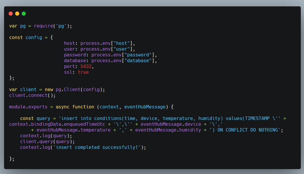
'insert into conditions(time, device, temperature, humidity) values(TIMESTAMP \'' + context.bindingData.enqueuedTimeUtc + '\',\'' + eventHubMessage.device + '\',' + eventHubMessage.temperature + ',' + eventHubMessage.humidity + ') ON CONFLICT DO NOTHING';
Notice the ON CONFLICT clause? When any constraint is violated, we do nothing. We do not add or modify data, we leave it all as it was.
The full Azure Function code is below:
Azure Function code with IoT Hub enqueuedTimeUtc and upsert
Conclusion
The above code is a little bit better already. We are not quite there yet but the two changes make sure that the date of the event is correct and independent from when the actual processing is done. By adding the constraint and upsert functionality, we make sure we do not end up with duplicate data when we reprocess data from IoT Hub.
In an earlier post, I looked at storing time-series data with TimescaleDB on Azure Database for PostgreSQL. To visualize your data, there are many options as listed here. Because TimescaleDB is built on PostgreSQL, you can use any tool that supports PostgreSQL such as Power BI or Tableau.
Grafana is a bit of a special case because TimescaleDB engineers actually built the data source, which is designed to take advantage of the time-series capabilities. For a detailed overview of the capabilities of the data source, see the Grafana documentation.
Let’s take a look at a simple example to get started. I have a hypertable called conditions with four columns: time, device, temperature, humidity. An IoT Simulator is constantly writing data for five devices: pg-1 to pg-5.
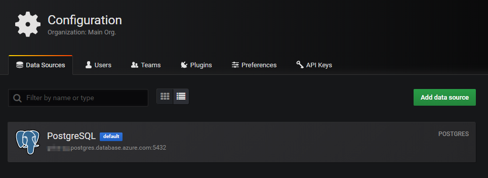
One setting in the data source is particularly noteworthy:
TimescaleDB support in the PostgreSQL datasource
Grafana has the concept of macro’s such as $_timeGroup or $_interval, as noted in the preceding image. The macro is translated to what the underlying data source supports. In this case, with TimescaleDB enabled, the macro results in the use of time_bucket, which is specific for TimescaleDB.
Creating a dashboard
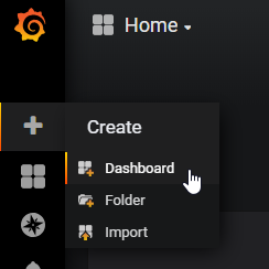
Create a dashboard from the main page:
Creating a new dashboard
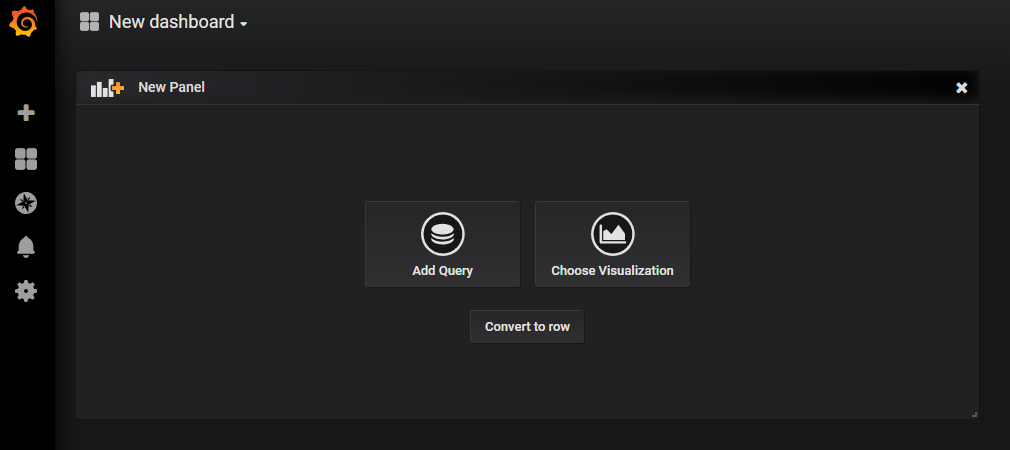
You will get a new dashboard with an empty panel:
Click Add Query. You will notice Grafana proposes a query. In this case it is very close because we only have one data source and table:
Grafana proposes the following query
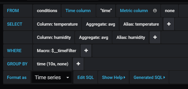
Let’s modify this a bit. In the top right corner, I switched the time interval to last 30 minutes. Because the default query uses WHERE Macro: $_timeFilter, only the last 30 minutes will be shown. That’s another example of a macro. I would like to show the average temperature over 10 second intervals. That is easy to do with a GROUP BY and $_interval. In GROUP BY, click the + and type or select time to use the time field. You will notice the following:
GROUP BY with $_interval
Just click $_interval and select 10s. Now add the humidity column to the SELECT statement:
Adding humidity
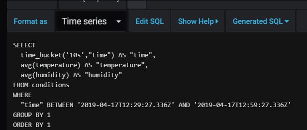
When you click the Generated SQL link, you will see the query built by the query builder:
Generated SQL
Notice that the query uses time_bucket. The GROUP BY 1 and ORDER BY 1 just means group and order on the first field which is the time_bucket. If the query builder is not sufficient, you can click Edit SQL and specify your query directly. When you switch back to query builder, your custom SQL statement might be overwritten if the builder does not support it.
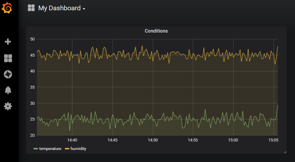
When you save your dashboard, you should see something like:
Pretty boring temperature and humidity graphWi
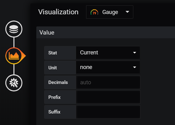
Now, let’s add a few gauges. In the top right row of icons, the first one should be Add panel. Choose the Gauge visualization and set your query:
Temperature Gauge
In Visualization, set Stat to Current:
Stat field on current
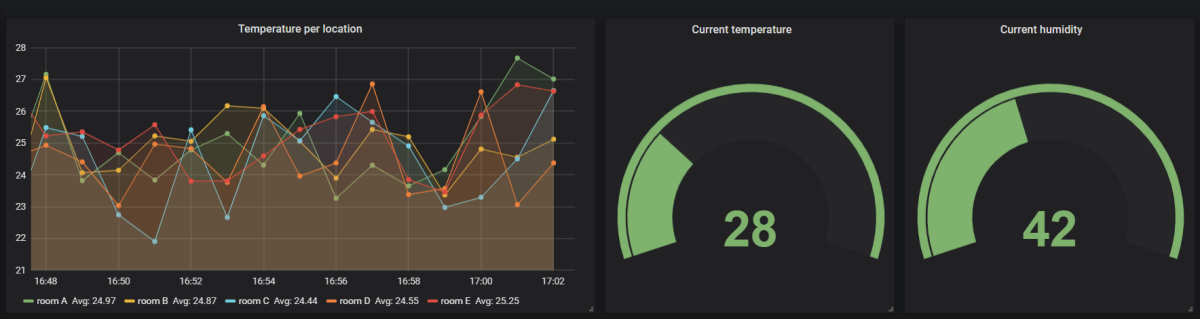
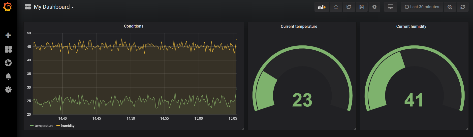
When the panel is finished, navigate back to the dashboard and duplicate the gauge. Modify the duplicated gauge to show humidity. Also change the titles. The dashboard now looks like:
Conditions dashboard
Grafana can be configured to auto refresh the dashboard. In the image below, refresh was set to every 5 seconds:
Setting auto refresh
Your dashboard will now update every 5 seconds for a more dynamic experience.
Joins
You can join hypertables with regular tables quite easily. This is one of the advantages of using a relational database such as PostgreSQL for your time-series data. The screenshot below shows a graph of the temperature per device location. The device location is stored in a regular table.
Join between hypertable and regular table: they are all just tables in the end
Here is the full dashboard:
Conclusion
Grafana, in combination with PostgreSQL and TimescaleDB, is a flexible solution for dashboarding your IoT time-series data. We have only scratched the surface here but it’s clear you can be up and running fast! Give it a go and tell me what you think in the comments or via @geertbaeke!
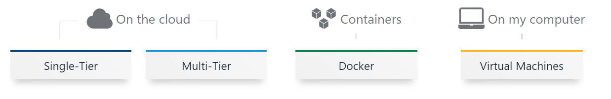
After seeing some tweets about Bitnami’s multi-tier Grafana Stack, I decided to give it a go. On the page describing the Grafana stack, there are several deployment offerings:
Grafana deployment offerings (Image: from Bitnami website)
I decided to use the multi-tier deployment, which deploys multiple Grafana nodes and a shared Azure Database for MariaDB.
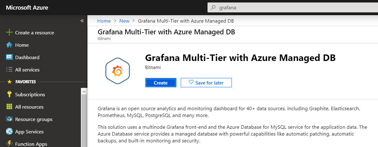
On Azure, the Grafana stack is deployed via an Azure Resource Manager (ARM) template. You can easily find it via the Azure Marketplace:
Grafana multi-tier in Azure Marketplace
From the above page, click Create to start deploying the template. You will get a series of straightforward questions such as the resource group, the Grafana admin password, MariaDB admin password, virtual machine size, etc…
It will take about half an hour to deploy the template. When finished, you will find the following resources in the resource group you chose or created during deployment:
Deployed Grafana resources
Let’s take a look at the deployed resources. The database back-end is Azure Database for MariaDB server. The deployment uses a General Purpose, 2 vCore, 50GB database. The monthly cost is around €130.
The Grafana VMs are Standard D1 v2 virtual machines (can be changed). These two machine cost around €100 per month. By default, these virtual machines have a public IP that allows SSH access on port 22. To logon, use the password or public key you configured during deployment.
To access the Grafana portal, Bitnami used an Azure Application Gateway. They used the Standard tier (not WAF) with the Medium SKU size and three nodes. The monthly cost for this setup is around €140.
The public IP address of the front-end can be found in the list of resources (e.g. in my case, mygrafanaagw-ip). The IP address will have an associated DNS name in the form of mygrafanaRANDOMTEXT-agw-dns.westeurope.cloudapp.azure.com. Simply connect to that URL to access your Grafana instance:
Grafana instance (after logging on and showing a simple dashboard
Naturally, you will want to access Grafana over SSL. That is something you will need to do yourself. For more information see this link.
It goes without saying that the template only takes care of deployment. Once deployed, you are responsible for the infrastructure! Security, backup, patching etc… is your responsibility!
Note that the template does not allow you to easily select the virtual network to deploy to. By default, the template creates a virtual network with address space 10.0.0.0/16. If you got some ARM templating skills, you can download the template right after validation but before deployment and modify it:
Downloading the template for modification
Conclusion
Setting up a multi-tier Grafana stack with Bitnami is very easy. Note that the cost of this deployment is around €370 per month though. Instead of deploying and managing Grafana yourself, you can also take a look at hosted offerings such as Grafana Cloud or Aiven Grafana.
In a previous post, I talked about saving time-series data to TimescaleDB, which is an extension on top of PostgreSQL. The post used an Azure Function with an Event Hub trigger to save the data in TimescaleDB with a regular INSERT INTO statement.
The Function App used the Windows runtime which gave me networking errors (ECONNRESET) when connecting to PostgreSQL. I often encounter those issues with the Windows runtime. In general, for Node.js, I try to stick to the Linux runtime whenever possible. In this post, we will try the same code but with a Function App that uses the Linux runtime in a Consumption Plan.
Make sure Azure CLI is installed and that you are logged in. First, create a Storage Account:
Now, in the Function App, set the following Application Settings. These settings will be used in the code we will deploy later.
host: hostname of the PostgreSQL server (e.g. servername.postgres.database.azure.com)
user: user name (e.g. user@servername)
password
database: name of the PostgreSQL database
EH: connection string to the Event Hub interface of your IoT Hub; if your are unsure how to set this, see this post
You can set the above values from the Azure Portal:
Application Settings of the Function App
The function uses the first four Application Settings in the function code via process.env:
Using Application Settings in JavaScript
The application setting EH is used to reference the Event Hub in function.json:
function.json with Event Hub details such as the connection, cardinality and the consumerGroup
Now let’s get the code from my GitHub repo in the Azure Function. First install Azure Function Core Tools 2.x. Next, create a folder called funcdemo. In that folder, run the following commands:
git clone https://github.com/gbaeke/pgfunc.git
cd pgfunc
npm install
az login
az account show
The npm install command installs the pg module as defined in package.json. The last two commands log you in and show the active subscription. Make sure that subscription contains the Function App you deployed above. Now run the following command:
func init
Answer the questions: we use Node and JavaScript. You should now have a local.settings.json file that sets the FUNCTIONS_WORKER_RUNTIME to node. If you do not have that, the next command will throw an error.
Now issue the following command to package and deploy the function to the Function App we created earlier:
func azure functionapp publish funclinux
This should result in the following feedback:
Feedback from function deployment
You should now see the function in the Function App:
Deployed function
To verify that the function works as expected, I started my IoT Simulator with 100 devices that send data every 5 seconds. I also deleted all the existing data from the TimescaleDB hypertable. The Live Metrics stream shows the results. In this case, the function is running smoothly without connection reset errors. The consumption plan spun up 4 servers:
Live Metrics Stream of IoT Hub to PostgreSQL function
In IoT projects, the same question always comes up: “Where do we store our telemetry data?”. As usual, the answer to that question is not straightforward. We have seen all kinds of solutions in the wild:
save directly to a relational database (SQL Server, MySQL, …)
save to a data lake and/or SQL
save to Cosmos DB or similar (e.g. MongoDB)
save to Azure Table Storage or similar
save to Time Series Insights
Saving the data to a relational database is often tempting. It fits in existing operational practices and it is easy to extract, transform and visualize the data. In practice, I often recommend against this approach except in the simplest of use cases. The reason is clear: these databases are not optimized for fast ingestion of time-series data. Instead, you should use a time-series database which is optimized for fast ingest and efficient processing of time-series data.
TimescaleDB
TimescaleDB is a an open-source time-series databases optimized for fast ingest even when the amount of data stored becomes large. It does not stand on its own, as it runs on PostgreSQL as an extension. Note that you can store time-series in a regular table or as a TimescaleDB hypertable. The graphic below (from this post), shows the difference:
Test on general purpose compute Gen 5 with 8 vCores, 45GB RAM with Premium Storage
The difference is clear. With a regular table, the insert rate is lowered dramatically when the amount of data becomes large.
The TimescaleDB extension can easily be installed on Azure Database for PostgreSQL. Let’s see how that goes shall we?
Installing TimescaleDB
To create an Azure Database for PostgreSQL instance, I will use the Azure CLI with the db-up extension:
az postgres up -g RESOURCEGROUP -s SERVERNAME -d DBNAME -u USER -p PASSWORD
The server name you provide should result in a unique URL for your database (e.g. servername.postgres.database.azure.com).
Tip: do not use admin as the user name 👍
When the server has been provisioned, modify the server confguration for the TimescaleDB extension:
az postgres server configuration set --resource-group RESOURCEGROUP ––server-name SERVERNAME --name shared_preload_libraries --value timescaledb
Now you need to actually install the extension. Install pgAdmin and issue the following query:
CREATE EXTENSION IF NOT EXISTS timescaledb CASCADE;
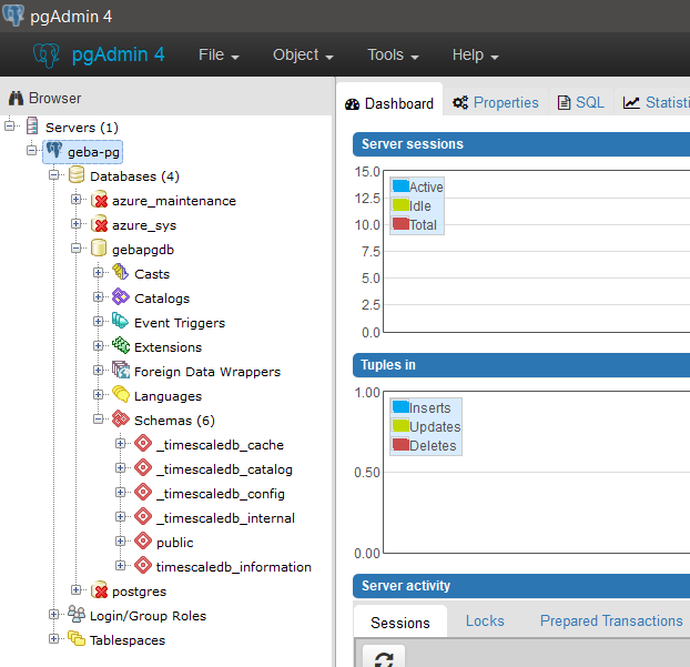
In pgAdmin, you should see extra schemas for TimescaleDB:
Extra schemas for TimescaleDB
Creating a hypertable
A hypertable uses partitioning to optimize writing and reading time-series data. Creating such a table is straightforward. You start with a regular table:
CREATE TABLE conditions (
   time        TIMESTAMPTZ       NOT NULL,
   location    TEXT              NOT NULL,
   temperature DOUBLE PRECISION  NULL,
   humidity    DOUBLE PRECISION  NULL );
Next, convert to a hypertable:
SELECT create_hypertable('conditions', 'time');
The above command partitions the data by time, using the values in the time column. By default, the time interval for partitioning is set to 7 days, starting from version 0.11.0 of TimescaleDB. You can override this by setting chunk_time_interval when creating the hypertable. You should make sure that the chunk belonging to the most recent interval can fit into memory. According to best practices, such a chunk should not use more than 25% of main memory.
Now that we have the hypertable, we can write time-series data to it. One advantage of being built on top of a relational database such as PostgreSQL is that you can use standard SQL INSERT INTO statements. For example:
The example above is from an Azure Function we will look at in a moment. In extracts values from a message received via IoT Hub and inserts them into the hypertable via an INSERT INTO query.
Let’s take a look at the Azure Function next.
Azure Function: from IoT Hub to the Hypertable
The Azure Function is kept bare bones to focus on the essentials. Note that you will need to open the console and install the pg module with the following command:
npm install pg
The image below shows the Azure Function (based on this although the article does not use a hypertable and stores the telemetry as JSON).
Bare bones Azure Function to write IoT Hub data to the hypertable
Naturally, the Azure Function above requires an Azure Event Hubs trigger. In this case, event hub cardinality was set to One. More information here. Note that you should NOT use the NOW() function to set the time. It’s only used here for demo purposes. Instead, you should take the timestamp sent by the device or the time the data was queued at the Event Hub!
Naturally, you will also need an IoT Hub where you send your data. In this case, I created a standard IoT Hub and used the IoT Hub Visual Studio Code extension to generate code (1 in image below) to send sample messages. I modified the code somewhat to include the device name (2 in image below):
Visual Studio toolkit used to create the device, generate code and modify the code
Now we can run the code (saved as sender.js) with:
node sender.js
Note: do not forget to first run npm install azure-iot-device
Data is being sent:
Data sent to IoT Hub
Data processed by the Azure Function as viewed in Application Insights Live Metrics stream:
Application Insights Live Metrics stream
With only one device sending data, there isn’t that much to do! In pgAdmin, you should see connections from at least one of the Azure Function hosts that are active:
Connections to PostgreSQL
Note: I encountered some issues with ECONNRESET errors under higher load; take a look at this post which runs the same function on a Linux Consumption Plan
Querying the data
TimescaleDB, with help from PostgreSQL, has a rich query language especially when compared to some other offerings. Yes, I am looking at you Cosmos DB! 😉 Below are some examples (based on the documentation at https://docs.timescale.com/v1.2/using-timescaledb/reading-data:
SELECT COUNT(*) FROM conditions WHERE time > NOW() - interval '1 minute';
The above query simply counts the messages in the last minute. Notice the flexibility in expressing the time which is what we want from time-series databases.
SELECT time_bucket('1 minute', time) AS one_min, device, COUNT(*), MAX(temperature) AS max_temp, MAX(humidity) AS max_hum FROM conditions WHERE time > NOW() - interval '10 minutes' GROUP BY one_min, device ORDER BY one_min DESC, max_temp DESC;
The above query displays the following result:
Conclusion
When dealing with time-series data, it is often beneficial to use a time-series database. They are optimized to ingest time-series data at high speed and greater efficiency than general purpose SQL or NoSQL databases. The fact that TimescaleDB is built on PostgreSQL means that it can take advantage of the flexibility and stability of PostgreSQL. Although there are many other time-series databases, TimescaleDB is easy to use when coupled with PaaS (platform-as-a-service) PostgreSQL offerings such as Azure Database for PostgreSQL.
In this short post, we will take a look at Cloud Run on Google Kubernetes Engine (GKE). To get this to work, you will need to deploy a Kubernetes cluster. Make sure you use nodes with at least 2 vCPUs and 7.5 GB of memory. Take a look here for more details. You will notice that you need to include Istio which will make the option to enable Cloud Run on GKE available.
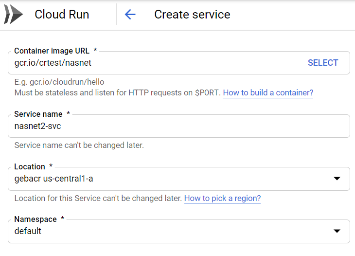
To create a Cloud Run service on GKE, navigate to Cloud Run in the console and click Create Service. For location, you can select your Kubernetes cluster. In the screenshot below, the default namespace of my cluster gebacr in zone us-central1-a was chosen:
Cloud Run service on GKE
In Connectivity, select external:
External connectivity to the service
In the optional settings, you can specify the allocated memory and maximum requests per container.
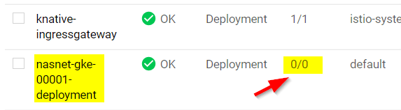
When finished, you will see a deployment on your cluster:
Cloud Run Kubernetes deployment (note that the Cloud Run service is nasnet-gke)
Notice that, like with Cloud Run without GKE, the deployment is scaled to zero when it is not in use!
To fix that, you can patch the domain name to something that can be resolved, for instance a xip.io address. First get the external IP of the istio-ingressgateway:
kubectl get service istio-ingressgateway --namespace istio-system
Next, patch the config-domain configmap to replace example.com with <EXTERNALIP>.xip.io
In my example Cloud Run service, I now get the following URL (not the actual IP):
http://nasnet-gke.default.107.198.183.182.xip.io/
Note: instead of patching the domain, you could also use curl to connect to the external IP of the ingress and pass the host header nasnet-gke.default.example.com.
With that URL, I can connect to the service. In case of a cold start (when the ReplicaSet has been scaled to 0), it takes a bit longer that “native” Cloud Run which takes a second or so.
It is clear that connecting to the Cloud Run service on GKE takes a bit more work than with “native” Cloud Run. Enabling HTTPS is also more of a pain on GKE where in “native” Cloud Run, you merely need to validate your domain and Google will configure a Let’s Encrypt certificate for the domain name you have configured. Cloud Run cold starts also seem faster.
That’s it for this quick look. In general, try to use Cloud Run versus Cloud Run on GKE as much as possible. Less fuss, more productivity! 😉
With the release of Google’s Cloud Run, I decided to check it out with my nasnet container.
With Cloud Run, you simply deploy your container and let Google scale it based on the requests it receives. When your container is not used, it gets scaled to zero. As such, it combines the properties of a serverless offering such as Azure Functions with standard containers. Today, you cannot put limits on scaling (e.g. max X instances).
You might be tempted to compare Cloud Run to something like Azure Container Instances but it is not exactly the same. True, Azure Container Instances (ACI) allows you to simply deploy a container without the need for an orchestrator such as Kubernetes. With ACI however, memory and CPU capacity are reserved and it does not scale your container based on the requests it receives. ACI can be used in conjunction with virtual nodes in AKS (Kubernetes on Azure) to achieve somewhat similar results at higher cost and complexity. However, ACI can be used in broader scenarios such as stateful applications beyond the simple HTTP use case.
Prerequisites
Cloud Run containers should be able to fit in 2GB of memory. They should be stateless and all computation should be scoped to a HTTP request.
Your container needs to be invocable via HTTP requests on port 8080. It is against best practices though to hardcode this port. Instead, you should check the PORT environment variable that is automatically injected into the container by Cloud Run. Google might change the port in the future! In the nasnet container, the code checks this as follows:
port := getEnv("PORT", "9090")
getEnv is a custom function that checks the environment variable. If it is not set, port is set to the value of the second parameter:
func getEnv(key, fallback string) string {
 value, exists := os.LookupEnv(key)
 if !exists {
  value = fallback
 }
 return value
}
Later, in the call to ListenAndServe, the port variable is used as follows:
log.Fatal(http.ListenAndServe(":"+port, nil))
Deploying to Cloud Run
Make sure you have access to Google Cloud and create a project. I created a project called CRTest.
Next, clone the nasnet-go repository:
git clone https://github.com/gbaeke/nasnet-go.git
If you have Docker installed, issue the following command to build and tag the container (from the nasnet-go folder which is a folder created by the git clone command above):
docker build -t gcr.io/<PROJECT>/nasnet:latest .
In the above command, replace <PROJECT> with your Google Cloud project name.
To push the container image to the Google Cloud Repository, install gcloud. When you run gcloud init, you will have to authenticate to Google Cloud. We install gcloud here to make the authentication process to Google Container Registry easier. To do that, run the following command:
gcloud auth configure-docker
Next, authenticate to the registry:
docker login gcr.io/<PROJECT>
Now that you are logged in, push the image:
docker push gcr.io/<PROJECT>/nasnet:latest
If you don’t want to bother yourself with local build and push, you can use Google Cloud Build instead:
gcloud builds submit --tag gcr.io/crtest/nasnet .
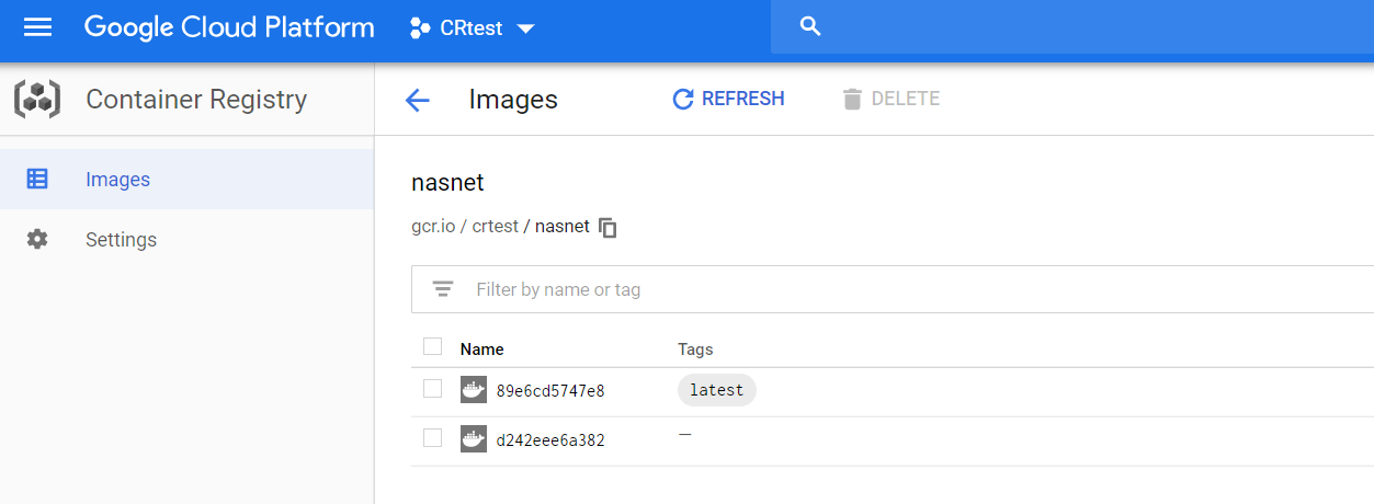
The above command will package you source files, submit them to Cloud Build and build the container in Google Cloud. When finished, the container image will be pushed to gcr.io/crtest. Either way, when the push is done, check the image in the console:
The nasnet container image in gcr
Now we have the image in the repository, we can use it with Cloud Run. In the console, navigate to Cloud Run and click Create Service:
Creating a Cloud Run service for nasnet
By default, allocated memory is set to 256MB which is too low for this image. Set allocated memory to 1GB. If you set it too low, your container will be restarted. Click Optional Settings and change the allocated memory:
Change the allocated memory for the nasnet container
Note: this particular container writes files you upload to the local file system; this is not recommended since data written to the file system is counted as memory
Note: the container will handle multiple requests up to a maximum of 80; currently 80 concurrent requests per container is the maximum
Now finish the configuration. The image will be pulled and the Cloud Run service will be started:
Cloud Run gives you a https URL to connect to your container. You can configure custom domains as well. When you browse to the URL, you should see the following:
Try it by uploading an image to classify it!
Conclusion
Google Cloud Run makes it easy to deploy HTTP invocable containers in a serverless fashion. In this example, I modified the nasnet code to check the PORT environment variable. In the runtime configuation, I set the amount of memory to 1GB. That was all that was needed to get this container to run. Note that Cloud Run can also be used in conjunction with GKE (Google Kubernetes Engine). That’s a post for some other time!
A while ago, I wrote a post about Azure Front Door. In that post, I wrote that http to https redirection was not possible. With Azure Front Door being GA, let’s take a look if that is still the case.
In the previous post, I had the following configuration in Front Door Designer:
Azure Front Door Designer
The above configuration exposes a static website hosted in an Azure Storage Acccount (the backend in the backend pool). The custom domain deploy.baeke.info maps to geba.azurefd.net using a CNAME in my CloudFlare hosted domain. The routing rule routeall maps all requests to the backend.
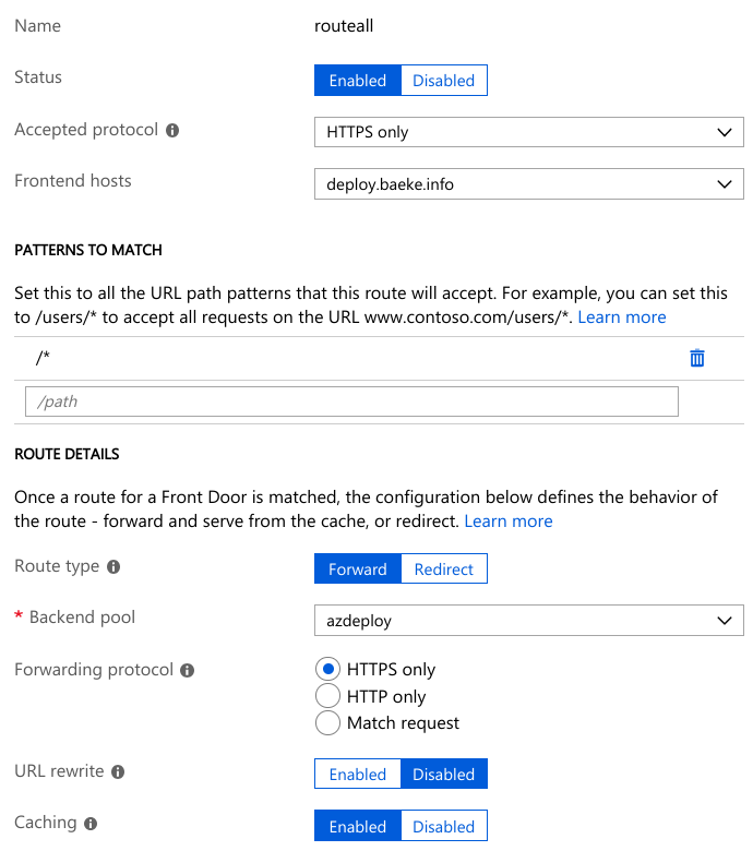
The above configuration does not, however, redirect http://deploy.baeke.info to https://deploy.baeke.info which is clearly not what we want. In order to achieve that goal, the routing rules can be changed. A redirect routing rule looks as follows:
Redirect routing rule (Replace destination host was not required)
The routall rule looks like this:
Routing rule
The routing rule simply routes https://deploy.baeke.info to the azdeploy backend pool which only contains the single static website hosted in a storage account.
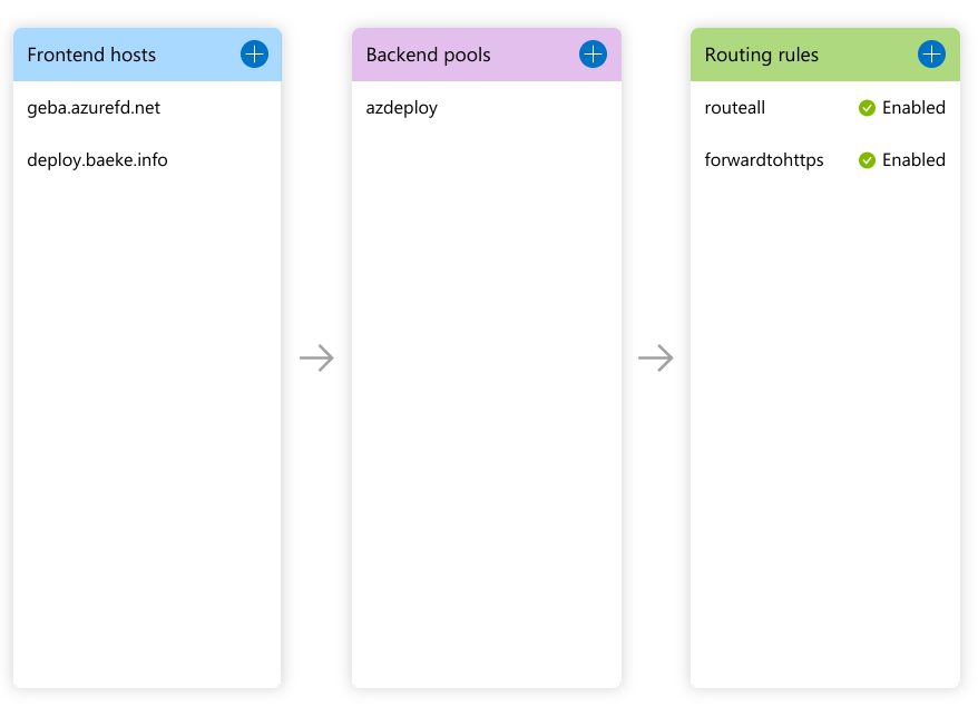
The full config looks like this:
Full config in Front Door designer
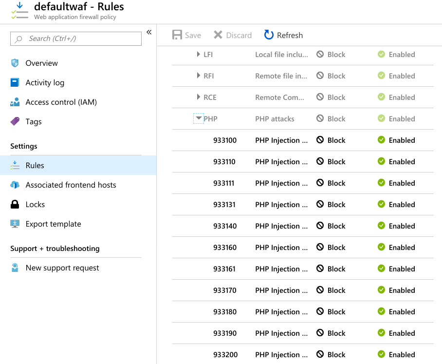
Although not very useful for this static website, I also added WAF (Web Application Firewall) rules to Azure Front Door. In the Azure Portal, just search for WAF and add a policy. I added a default policy and associated it with this Azure Front Door website:
WAF rules associated with the Azure Front Door frontend